Forecasting the Unthinkable: Sequential Modelling and Early Warning Systems
Humanitarian emergencies rarely strike without warning. They accumulate through the slow compounding of climate shocks, economic volatility, and social conflict over months and years. By treating the data as dynamic temporal sequences rather than static snapshots, Project HERO extracts predictive signals that can anticipate the deterioration of food security before a crisis reaches its apex.
Target Variable Definition — IPC Phase 3+: The primary target metric analyzed throughout our time-series and forecasting models is the IPC Phase 3+ proportion. Based on the Integrated Food Security Phase Classification (IPC) standard, IPC 3+ measures the percentage of population living under Acute Food Insecurity — combining Crisis (Phase 3), Emergency (Phase 4), and Catastrophe/Famine (Phase 5).
📍 Case Study: Badakhshan Province, Afghanistan (ADM1: AF17)
Throughout this page we illustrate the full TSA pipeline on Badakhshan, a remote mountainous province in north-eastern Afghanistan chronically affected by food insecurity. The same battery of analyses (decomposition, autocorrelation, anomaly detection, and multi-model forecasting) has been applied systematically to every ADM1 region across all countries in the HERO dataset.
1. The First Challenge: Temporal Misalignment
The raw data arrives fragmented across incompatible timescales. Conflict events from ACLED are recorded daily. WFP price readings come weekly. IPC food security assessments happen sporadically, sometimes months apart. Feeding these into a coherent forecasting system requires careful temporal harmonisation.
Forecast & Anomaly Detection Pipeline
Ingestion & Alignment
WFP, ACLED, CHIRPS, IPC temporal re-gridding (Monthly MS)
Signal Decomposition
STL LOESS decomposition into Trend, Seasonality & Residuals
Feature & Anomaly Profiling
tsfresh metrics & Matrix Profile (Motifs & Discords)
Multi-Layer Forecasting
SARIMAX, Causal VAR, DTW Transfer & TimesFM Zero-Shot
2. Signal Engineering: Distilling the Mathematics of a Crisis
For each province, HERO computes a rich tsfresh feature vector, representing the mathematical signature of how that region’s indicators have evolved over time.
Skewness & Kurtosis
Measure whether a province's food security distribution skews toward extremes, serving as a key signature of structural fragility versus transient stress.
Hurst Exponent
The Hurst exponent H quantifies long-term memory: does a drought shock fade quickly, or does it compound over the following seasons?
Approximate Entropy
ApEn measures signal irregularity: high entropy signals unpredictable, chaotic conditions, while low entropy signals structural trends amenable to forecasting.
3. Decomposing the Signal: Separating Trend from Noise
Before forecasting, each time series is structurally decomposed using STL (Seasonal and Trend decomposition using LOESS), a regression-based method specifically chosen for its robustness to the massive outlier presence typical of conflict zones.
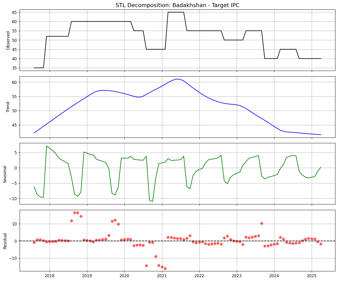
STL Decomposition of Badakhshan's IPC Phase 3+ acute food insecurity target (2017–2025). The trend peaked at ~60% during 2019–2021, coinciding with the Taliban takeover and successive drought seasons. Seasonal oscillations of ±10 pp reflect the lean season cycle. Residual spikes flag the shocks the model cannot predict from structure alone.
What STL Reveals
📈 Trend
The underlying long-run trajectory of food insecurity, stripped of seasonal and random fluctuation.
🌀 Seasonality
Recurring annual patterns, such as harvest cycles, rainy seasons, and lean periods, isolated and modelled independently.
⚡ Residuals
The unexplained remainder, representing the space where systemic shocks hide. This is where the Matrix Profile operates.
4. Temporal Memory: Autocorrelation and Cross-Correlation Analysis
Understanding how quickly a signal forgets its own past, and how strongly different drivers lead or follow the target, is critical to selecting the right forecasting model.
ACF & PACF of the Differenced IPC Series
Reading the Correlogram
After first-order differencing (d=1), the IPC Phase 3+ target series for Badakhshan shows no significant autocorrelation at any lag, as all coefficients fall within the 95% confidence band. This means the differenced series behaves like white noise: the original signal is well-described by a simple random walk with drift, and any remaining predictive power must come from exogenous variables rather than the series' own history.
The PACF confirms this with a clean cut-off after lag 0, leaving no partial correlation structure to exploit, which presents a strong argument for moving beyond pure ARIMA toward multivariate models (VAR) or transfer learning approaches.
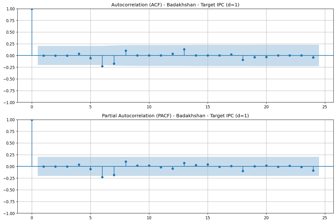
ACF (top) and PACF (bottom) of the first-differenced IPC Phase 3+ target series. No lag exceeds the 95% significance threshold, confirming near-white-noise behaviour after differencing.
Multi-Variable Autocorrelation Comparison
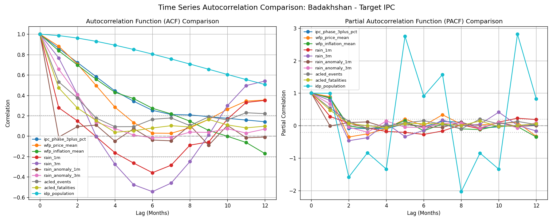
Autocorrelation (ACF) and Partial Autocorrelation (PACF) comparison across all 11 driver variables for Badakhshan. IPC Phase 3+ and IDP population exhibit the strongest long-memory persistence (ACF decaying slowly over 12+ months), while rainfall anomalies decay rapidly, suggesting they act as short-horizon triggers rather than sustained drivers.
Cross-Correlation with the IPC Target
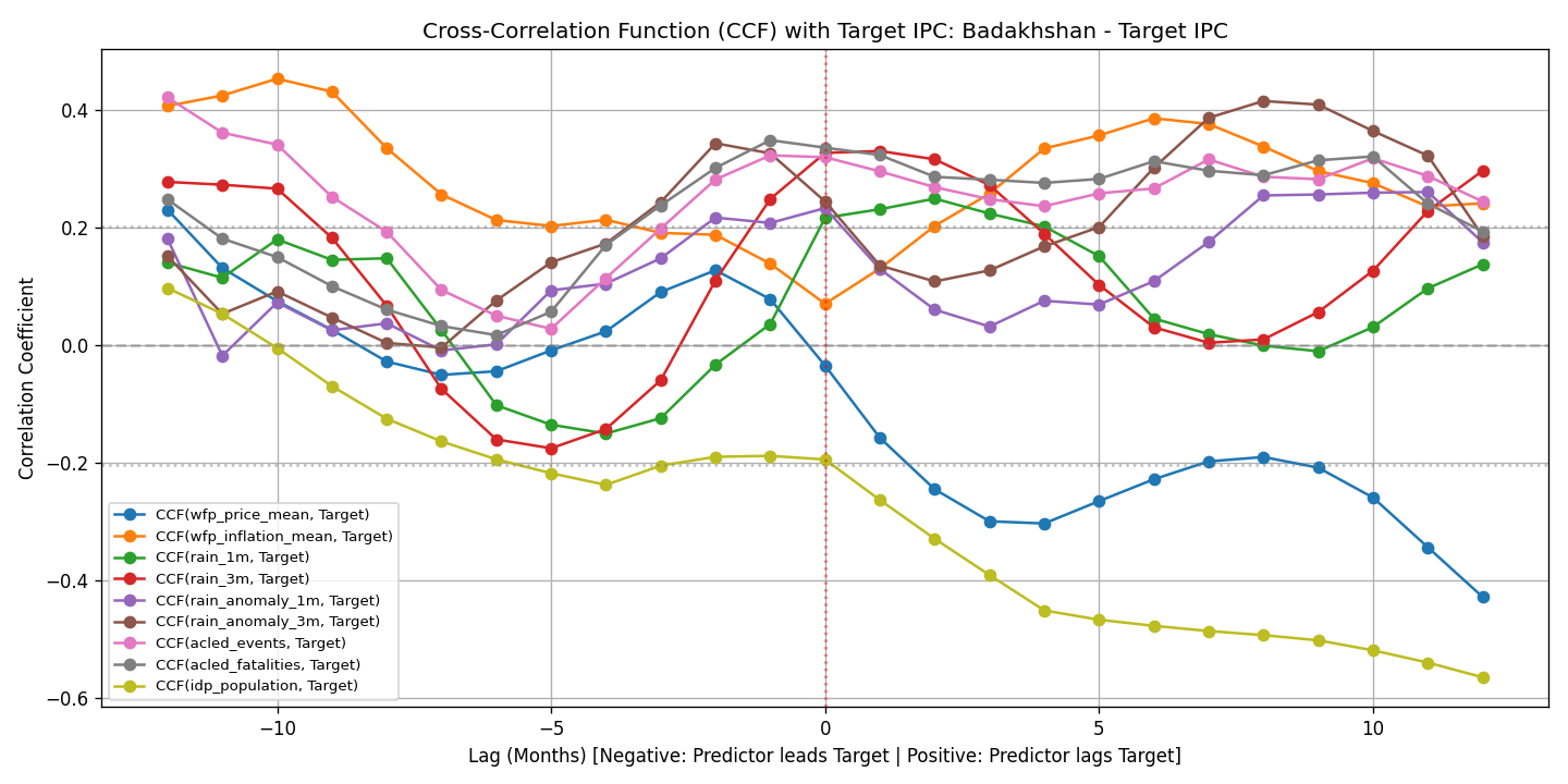
Cross-Correlation Function (CCF) between each driver and the IPC Phase 3+ target. Negative lags (left of the red line) indicate that the predictor leads the target, providing a direct measure of early warning potential.
Key Lead-Lag Insights
WFP inflation shows the strongest leading signal at lags −8 to −10 months (CCF ≈ 0.45), confirming that food price inflation precedes IPC Phase 3+ deterioration by nearly a year in Badakhshan.
Rainfall anomalies (3-month) peak at positive lags (+5 to +10), meaning they are lagging indicators where the drought effect materialises in the IPC Phase 3+ assessment only several months after the rainfall deficit occurs.
IDP population has the most asymmetric CCF profile: displacement drives future IPC worsening at all lead horizons, but the reverse effect decays rapidly.
5. Anomaly Detection via Matrix Profile
Stochastic residuals from the STL decomposition are analysed using the Matrix Profile algorithm, which scans the time series for two types of structural patterns.
📊 Data Availability for Reliable Anomaly Detection
The Matrix Profile operates on the IPC Phase 3+ target series, representing the percentage of population in acute food insecurity, after STL residual extraction. For each ADM1 region, the input data is assembled from:
IPC Assessments
Sporadic (2–4 per year per country). Re-gridded to monthly frequency via forward-fill interpolation. Coverage spans 2017–2025, yielding ~80–96 monthly observations per region, providing the minimum viable length for subsequence-based algorithms.
Exogenous Drivers (for context)
WFP prices (weekly → monthly), ACLED conflict events (daily → monthly), CHIRPS rainfall (dekadal → monthly), NDVI vegetation (bi-weekly → monthly), IDP displacement (monthly). These are used in the cross-correlation analysis to interpret the anomalies detected.
Reliability Constraints
Matrix Profile requires at least 3× the subsequence length in total observations. With a typical window of 6–12 months, the minimum threshold is ~36 months of data. Regions with fewer than 30 valid IPC observations are flagged as insufficient and excluded from anomaly detection.
| Pattern | Definition | Humanitarian Meaning |
|---|---|---|
| Motifs | Subsequences that recur frequently | Early warning signatures that precede IPC downgrade events |
| Discords | Subsequences that never recur | Isolated systemic shocks, such as conflict escalations and harvest collapses |
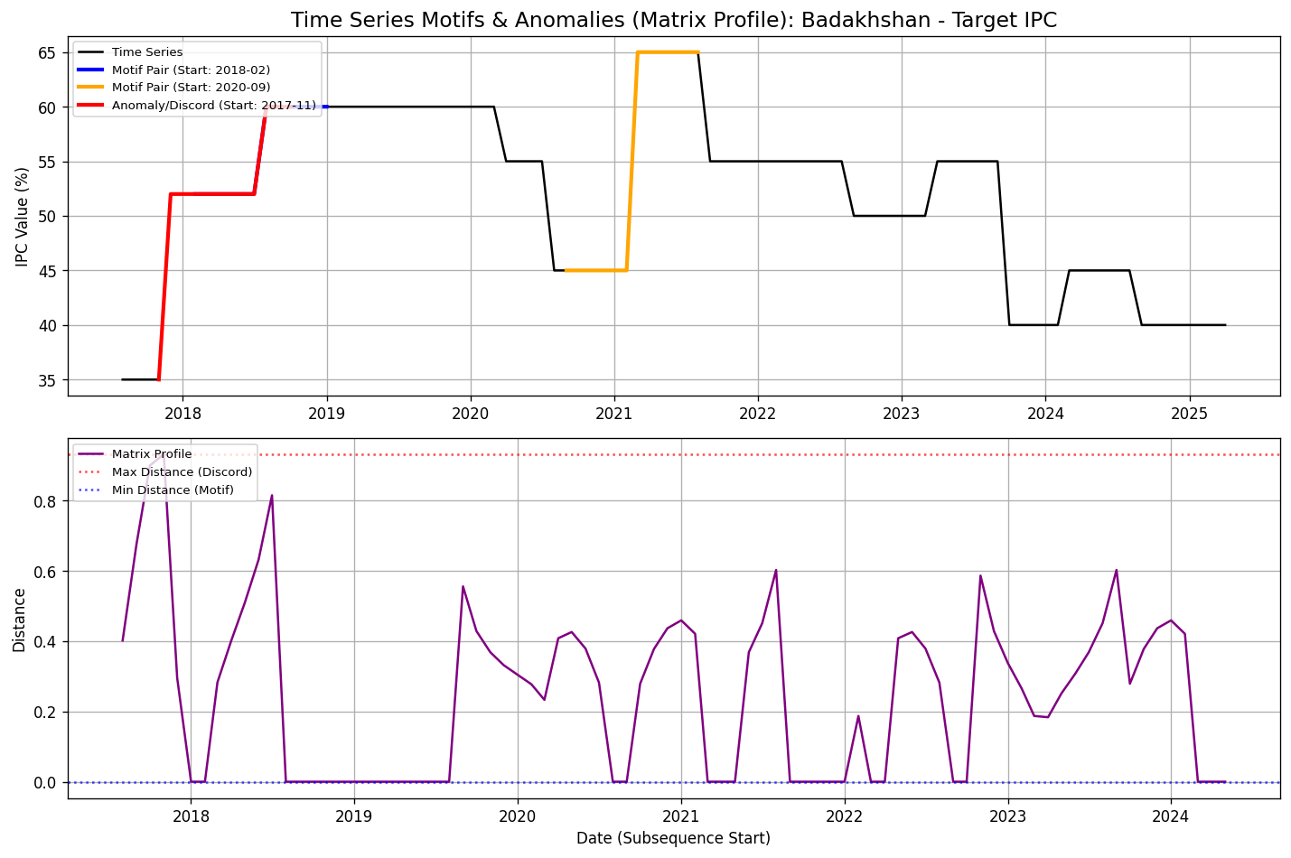
Top panel: the original IPC Phase 3+ time series with motif pairs (blue, orange) and the detected discord (red) highlighted. Bottom panel: the Matrix Profile distance function, where peaks represent anomalous subsequences and valleys represent recurring motifs.
What the Algorithm Found
Discord (Nov 2017): The rapid initial surge from ~35% to ~52% IPC Phase 3+ in late 2017 is flagged as the most anomalous subsequence in the entire record, marking a sudden regime shift with no historical precedent.
Motif Pair: The 2018–2019 plateau phase (blue) and the 2020–2021 spike (orange) share structural similarity, as both show a rapid rise followed by a sustained high plateau. This recurrence pattern can serve as an early warning template.
Residuals exceeding a critical threshold (Z-score > 2.0) are mapped onto a multi-provincial Anomaly Matrix heatmap, visually revealing the spatial and temporal alignment of socio-economic collapses across regions.
6. Forecasting Architecture: Four Layers of Prediction
No single model works everywhere. HERO uses a stratified forecasting framework that adapts to the data quality and structural context of each province.
Layer 1: Univariate Baselines
SARIMAX / Holt-Winters models are trained at ADM1/ADM2 level to capture pure autocorrelation patterns in the IPC Phase 3+ series. They set a performance benchmark for all more complex approaches.
Layer 2: Causal VAR
Vector Autoregression captures cross-variable feedback loops: a conflict escalation that destroys agricultural infrastructure generating food price inflation and worsening IPC Phase 3+ in the following months.
Layer 3: DTW Clustering + Transfer Learning
In conflict zones with fragmented data, Dynamic Time Warping clusters provinces with similar IPC Phase 3+ crisis trajectories. Joint models trained on clusters are highly resistant to overfitting on thin historical records.
Layer 4: TimesFM (Zero-Shot)
In areas with total data blackout, HERO tests Google's TimesFM foundation model to generate exploratory projections of IPC Phase 3+ without any local historical retraining, serving as the last resort for the most opaque crisis contexts.
Multi-Model Forecast Comparison
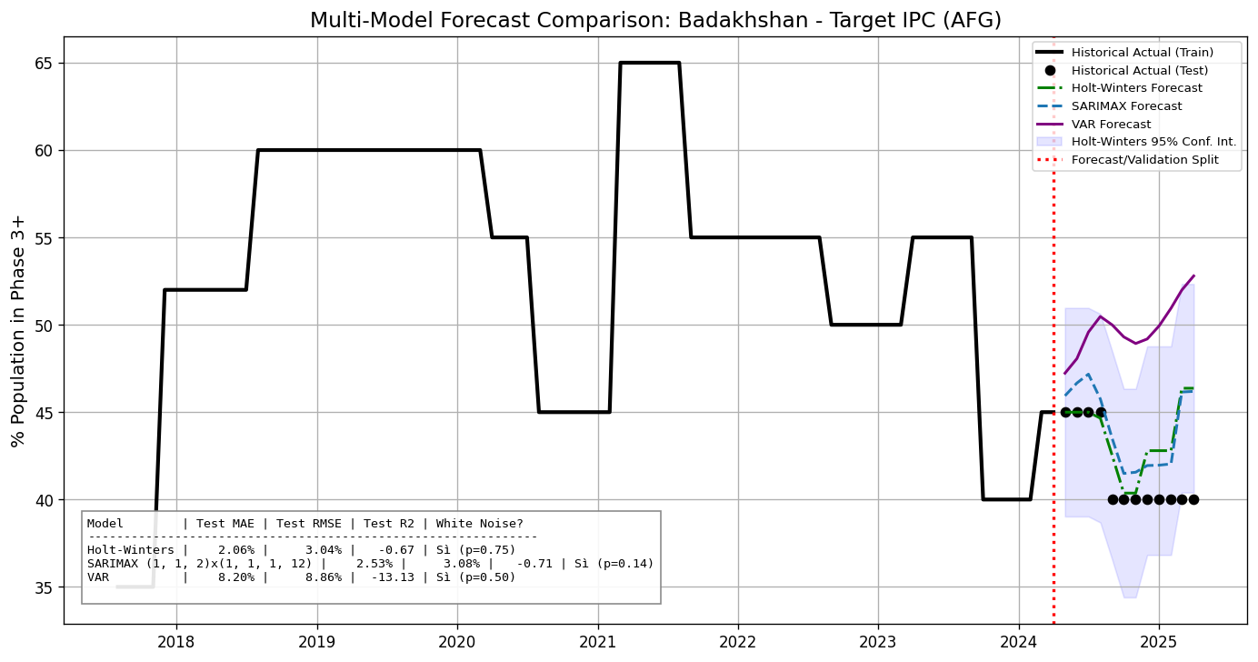
Holt-Winters (green), SARIMAX (blue dashed), and VAR (purple) forecasts of IPC Phase 3+ against the held-out test set (black dots). The red dashed line marks the train/test split point (2024). The light purple band shows the Holt-Winters 95% confidence interval.
Model Performance: Badakhshan
| Model | MAE | RMSE | R² |
|---|---|---|---|
| Holt-Winters | 2.06% | 3.04% | −0.67 |
| SARIMAX | 2.53% | 3.08% | −0.71 |
| VAR | 8.20% | 8.86% | −13.13 |
Both univariate baselines achieve MAE around 2–3 pp, closely tracking the test data. The VAR model diverges, as its multivariate feedback structure captures macro-dynamics well but overfits on Badakhshan's short history. Both Holt-Winters and SARIMAX pass the Ljung-Box white noise test on residuals (p > 0.05).
SARIMAX Order Selection (AIC/BIC)
Why ARIMA(1,1,2)×(1,1,1,12)?
HERO systematically evaluates multiple SARIMAX parameter combinations using the dual information criterion approach: AIC (Akaike) for predictive accuracy and BIC (Bayesian) for parsimony.
For Badakhshan, adding a seasonal component with period 12 dramatically reduces both criteria (from ~450 to ~320), confirming the annual lean-season cycle embedded in the IPC Phase 3+ signal. The final selected order ARIMA(1,1,2)×(1,1,1,12) achieves the lowest AIC while remaining within 5 points of the BIC minimum, balancing fit quality against model complexity.
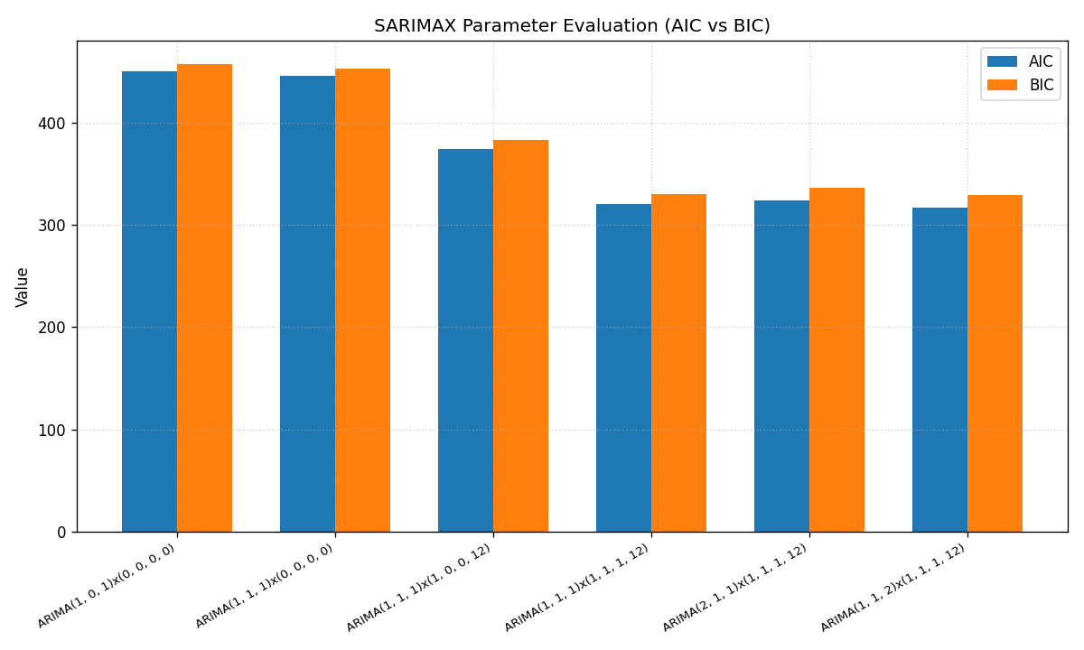
AIC (blue) and BIC (orange) across 6 candidate SARIMAX orders. Non-seasonal models (left) score substantially higher (~450), while seasonal models with s=12 (right three) cluster around 320–330, confirming the presence of a strong 12-month cycle in the IPC Phase 3+ series.
Residual Diagnostics
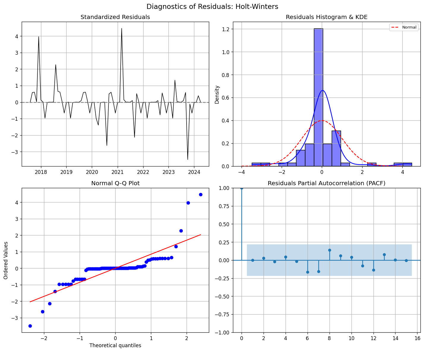
Four-panel diagnostic suite for the Holt-Winters model: standardised IPC Phase 3+ residuals over time (top-left), residual histogram with KDE and Normal overlay (top-right), Normal Q-Q plot (bottom-left), and residuals PACF (bottom-right).
Diagnostic Interpretation
Residual time series: The standardised residuals oscillate around zero without visible trend, though isolated spikes (2018, 2021, 2024) flag the same systemic shocks identified by the Matrix Profile.
Q-Q plot: Heavy tails at both extremes reveal that the residuals are leptokurtic, indicating that the model underestimates extreme events, a known challenge in conflict-affected forecasting.
PACF of residuals: All partial autocorrelations fall within the significance band, confirming the model has extracted all available temporal structure, as the residuals are white noise.
🌍 Reproducibility Note: The complete TSA pipeline shown above for Badakhshan (Afghanistan), including STL decomposition, ACF/PACF analysis, cross-correlation, Matrix Profile anomaly detection, SARIMAX order selection, multi-model forecasting, and residual diagnostics, is automatically executed for every ADM1 administrative region across all countries in the HERO dataset. All outputs are archived and accessible via the HERO Dashboard's TSA Diagnostics tab.